What are the sieve sizes for particle size distribution? A Guide to ASTM and ISO Standards

Sieve sizes are not arbitrary; they are part of a standardized system based on the number of openings per linear inch or the precise size of those openings in millimeters (mm) or micrometers (µm). While there isn't a single universal list, sizes are defined by standards like ASTM E11 (in the U.S.) and ISO 3310, which provide a consistent series of wire mesh sieves for accurate particle size analysis. A higher "mesh number" indicates more openings per inch, and therefore, smaller openings for finer particles.

The key to understanding sieve sizes is realizing they are tools used in a series, or a "stack." The goal isn't to find one specific size, but to select a standardized progression of sizes that work together to separate a material into distinct fractions, revealing its complete particle size distribution.

How Sieve Sizes Are Defined

To perform a particle size analysis, you must first understand the language used to describe the sieves themselves. This system is based on a clear, inverse relationship between the mesh number and the opening size.

The Concept of Mesh Number

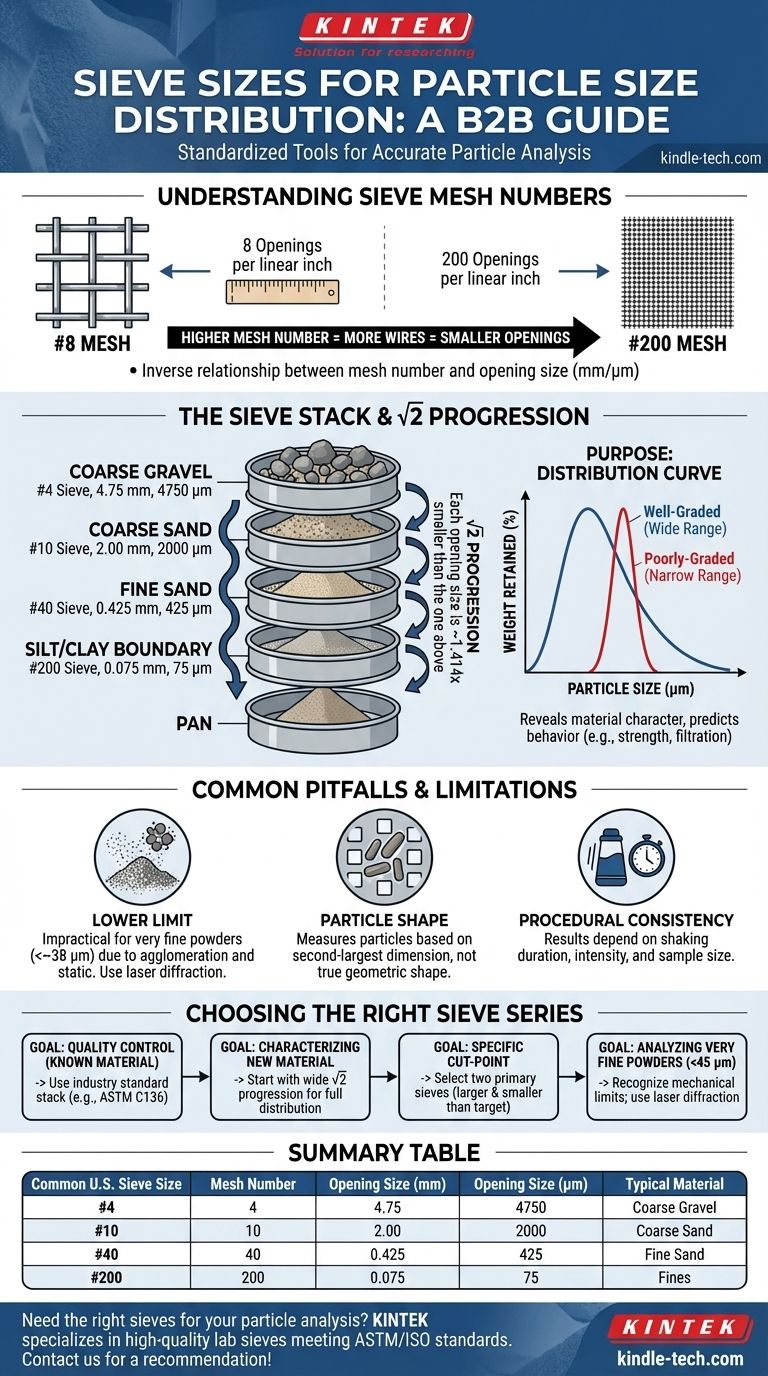
A sieve's mesh number refers to the number of openings in the wire mesh screen across one linear inch.

For example, a #8 mesh sieve has eight openings per inch. A #200 mesh sieve has 200 openings per inch.

Therefore, a higher mesh number means more wires, more openings, and consequently smaller openings.

From Mesh to Microns and Millimeters

Each standard mesh number corresponds to a specific opening size, typically measured in millimeters (mm) or micrometers (µm). One millimeter is equal to 1000 micrometers.

Here are a few common U.S. Standard sieve sizes to illustrate the relationship:

• #4 Sieve: 4.75 mm opening (coarse gravel)
• #10 Sieve: 2.00 mm opening (coarse sand)
• #40 Sieve: 425 µm opening (fine sand)
• #200 Sieve: 75 µm opening (silt and clay boundary)

As you can see, the mesh number and opening size have an inverse relationship.

Key Standardization Bodies

Sieve dimensions are governed by official standards to ensure results are repeatable and comparable across different labs.

The two dominant standards are ASTM E11 (common in the United States) and ISO 3310 (the international standard). While largely harmonized, it's critical to use sieves from the same standard within a single analysis.

Building a Sieve Stack for Analysis

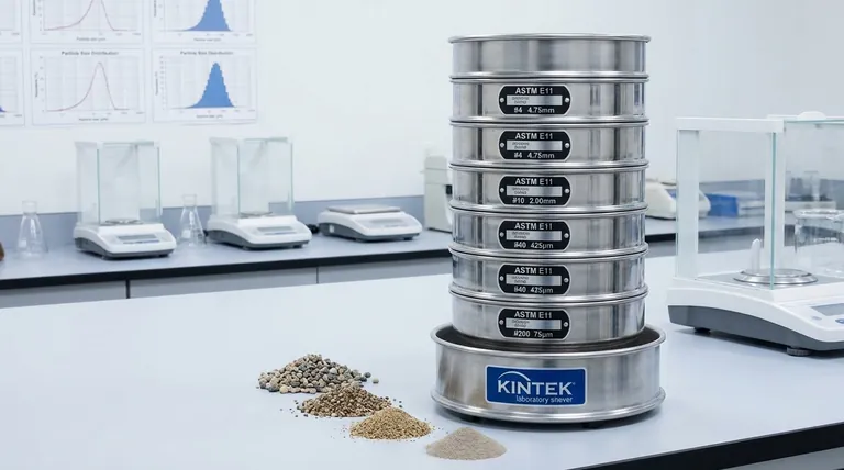
The real power of sieving comes from using multiple sieves stacked together, from the largest opening on top to the smallest on the bottom, with a solid pan at the very end to collect the finest particles.

The Goal: A Distribution Curve

The purpose of a sieve stack is to divide a sample by weight into different size fractions. By weighing the material retained on each sieve, you can generate a particle size distribution curve.

This curve is what reveals the character of your material—whether it's well-graded (a wide range of sizes) or poorly-graded (a narrow range of sizes). This distribution is critical for predicting a material's behavior, such as its strength in concrete, its filtration capacity, or its miscibility.

The √2 Progression

The most common and technically sound method for selecting sieves for a stack is to use a √2 (square root of 2) progression.

In this system, the opening size of each successive sieve in the series is approximately 1.414 times smaller than the sieve above it. This creates evenly spaced data points when plotted on a logarithmic scale, providing a clear and accurate picture of the distribution.

Common Pitfalls and Limitations

While sieve analysis is a straightforward and reliable method, it's essential to understand its limitations to ensure accurate interpretation.

The Lower Limit of Sieving

Sieve analysis becomes impractical and inaccurate for very fine powders. Particles smaller than ~38 micrometers (#400 mesh) tend to agglomerate, stick to the mesh wires due to static electricity, and resist passing through the openings.

For these fine materials, other methods like static light scattering (laser diffraction) or dynamic light scattering are required.

The Influence of Particle Shape

Sieving inherently measures a particle based on its second-largest dimension. An elongated or flat particle (like a sliver of rock) may pass through a mesh opening that is smaller than its total length.

This means sieve analysis provides a distribution based on a particle's ability to pass through a square hole, which may not represent its true geometric shape or volume.

Procedural Consistency is Key

The results of a sieve analysis are highly dependent on the procedure. Factors like the duration of shaking, the intensity of the shaking motion, and the initial sample size can all affect the final distribution. For results to be comparable, the procedure must be consistent.

How to Select the Right Sieve Series

Choosing the correct sieves depends entirely on the material you are analyzing and the question you need to answer.

• If your primary focus is quality control for a known material: Use the established standard sieve stack specified in your industry's test method (e.g., ASTM C136 for aggregates) to ensure compliance.
• If your primary focus is characterizing a new or unknown material: Start with a wide range of sieves in a √2 progression to capture the full distribution before refining your selection for future tests.
• If your primary focus is separating a material at a specific cut-point: Select two primary sieves—one just larger and one just smaller than your target particle size—to isolate your desired fraction efficiently.
• If your primary focus is analyzing very fine powders (below ~45 µm): Recognize the limits of mechanical sieving and choose an alternative method like laser diffraction for reliable results.

Ultimately, a thoughtful selection of sieve sizes transforms a simple separation test into a powerful tool for predicting and controlling material performance.

Summary Table:

Common U.S. Sieve Size	Mesh Number	Opening Size (mm)	Opening Size (µm)	Typical Material
Coarse Gravel	#4	4.75 mm	4750 µm	Gravel
Coarse Sand	#10	2.00 mm	2000 µm	Sand
Fine Sand	#40	0.425 mm	425 µm	Sand
Silt/Clay Boundary	#200	0.075 mm	75 µm	Fines

Need the right sieves for your particle analysis? KINTEK specializes in high-quality lab sieves and equipment that meet ASTM and ISO standards. Whether you're performing quality control on aggregates or characterizing a new material, our sieves deliver the accuracy and repeatability your lab demands. Contact our experts today to discuss your specific application and get a recommendation for the perfect sieve stack!